Exploring a stellarator

This tutorial loads one stellarator and plots its main characteristics: the plasma boundary, \(\lvert B \rvert\) on a flux surface, the boundary rebuilt from its Fourier modes, its alpha-particle losses, and the heat flux those losses put on the plasma boundary.

First install the pip package:

pip install boss-bench

Load a stellarator

There are two types of data files in the BoSS: trajectory files, containing guiding-center trajectory data, and confinement files, containing the initial and final states of fast ions. This tutorial will pull data from a confinement file, confinement_data_test_split_00000.hdf5.

Download this file from the Download Data page into a folder, here BoSS/. Each confinement file holds about 3,000 stellarators, and every field is an HDF5 dataset whose first axis runs over them, so row i of every dataset belongs to stellarator i.

import h5py
import matplotlib.pyplot as plt
import numpy as np

import boss_bench as bb

# take the first confinement file of the test split
path = bb.list_files("BoSS", "confinement", "test")[0]
f = h5py.File(path, "r")
print(len(f["uuid"]), "stellarators in", path)

load_record() reads every field of one stellarator into a dict. Give it the row of the stellarator, or its uuid:

# read every field of stellarator 0 into a dict
rec = bb.load_record(f, 0)
nfp = int(rec["nfp"])
print(rec["uuid"], "| source:", rec["source_dataset"], "| nfp =", nfp,
      f"| aspect ratio = {rec['aspect_ratio']:.2f} | beta = {rec['plasma_beta']:.4f}")

Gridded fields are stored flattened. Reshape them as described in grids and array shapes:

modB_boozer = rec["modB_boozer"].reshape(15, 41, 41)   # (s, zeta, theta), Boozer angles
boundary    = rec["boundary_xyz"].reshape(41, 41, 3)   # (phi, theta, xyz), one field period

The plasma boundary

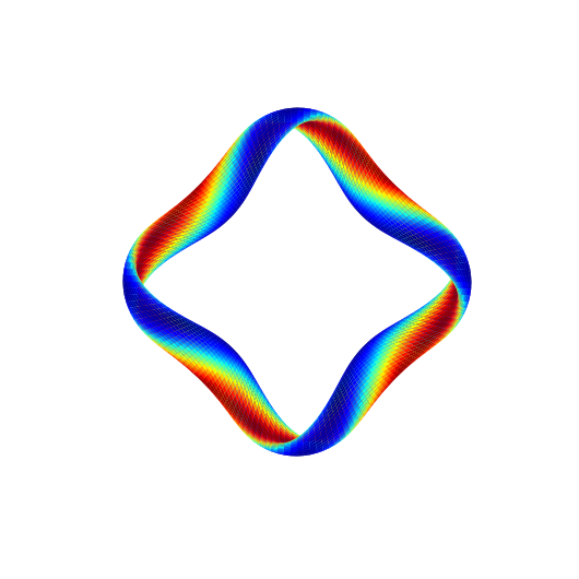
boundary_xyz covers one field period. plot_device() copies it around the torus and draws the whole boundary, colored by \(\lvert B \rvert\) and viewed from above:

bb.plot_device(rec)

|B| on a flux surface

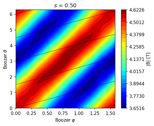
In Boozer coordinates a quasi-symmetric stellarator has straight \(\lvert B \rvert\) contours, and a quasi-isodynamic one has poloidally closed contours. plot_modB_boozer() draws \(\lvert B \rvert\) on the stored flux surface nearest to \(s\), with field lines in black:

bb.plot_modB_boozer(rec, s=0.5)

The boundary from its Fourier modes

boundary_xyz is sampled on a fixed 41 × 41 grid. For a finer surface, or for normals and curvature, load the Fourier modes in boundary_full_res_fourier_modes into a SIMSOPT SurfaceRZFourier (boundary Fourier modes describes the layout):

pip install simsopt

from simsopt.geo import SurfaceRZFourier

def boundary_surface(rec, phi, theta):
    """The plasma boundary as a SIMSOPT surface, at angles phi and theta in turns."""
    surface = SurfaceRZFourier(nfp=int(rec["nfp"]), stellsym=True, mpol=20, ntor=20,
                               quadpoints_phi=phi, quadpoints_theta=theta)
    surface.x = rec["boundary_full_res_fourier_modes"]
    return surface

# on the stored grid it reproduces boundary_xyz
surface = boundary_surface(rec, rec["boundary_quadpoints_phi"], rec["boundary_quadpoints_theta"])
print("max |difference| from boundary_xyz:", np.abs(surface.gamma() - boundary).max())

# a fine grid over the full torus
fine = boundary_surface(rec, np.linspace(0, 1, 200, endpoint=False), np.linspace(0, 1, 64, endpoint=False))
xyz = fine.gamma()            # (200, 64, 3) points on the boundary
normals = fine.unitnormal()   # (200, 64, 3) unit normals

Alpha-particle losses

The stellarator has 15,000 alpha particles, 5,000 born on each of the surfaces \(s_0 = 0.1\), \(0.25\) and \(0.5\). A particle is lost if its confinement_time is shorter than the simulation time t_max. Loss quantities are computed over the particles born on one surface:

# per particle: time it was lost (t_max if never lost) and its birth surface
ct, t_max, s_init = rec["confinement_time"], rec["t_max"], rec["s_init"]
for s0 in (0.1, 0.25, 0.5):
    print(f"born on s = {s0}: "
          f"loss fraction {bb.loss_fraction(ct, t_max, s_init, s0):.3f}, "
          f"normalized energy loss {bb.normalized_energy_loss(ct, t_max, s_init, s0):.3f}")

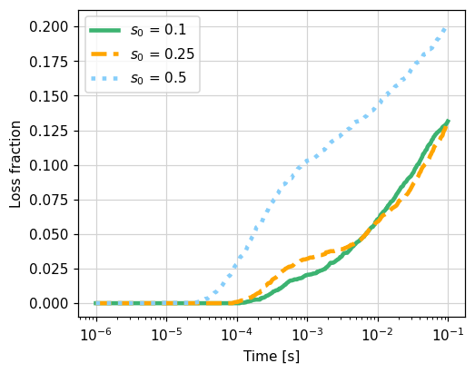
The fraction of particles lost by time \(t\) shows how quickly they are lost. Particles born closer to the edge are lost sooner:

bb.plot_loss_fraction_curves(rec)

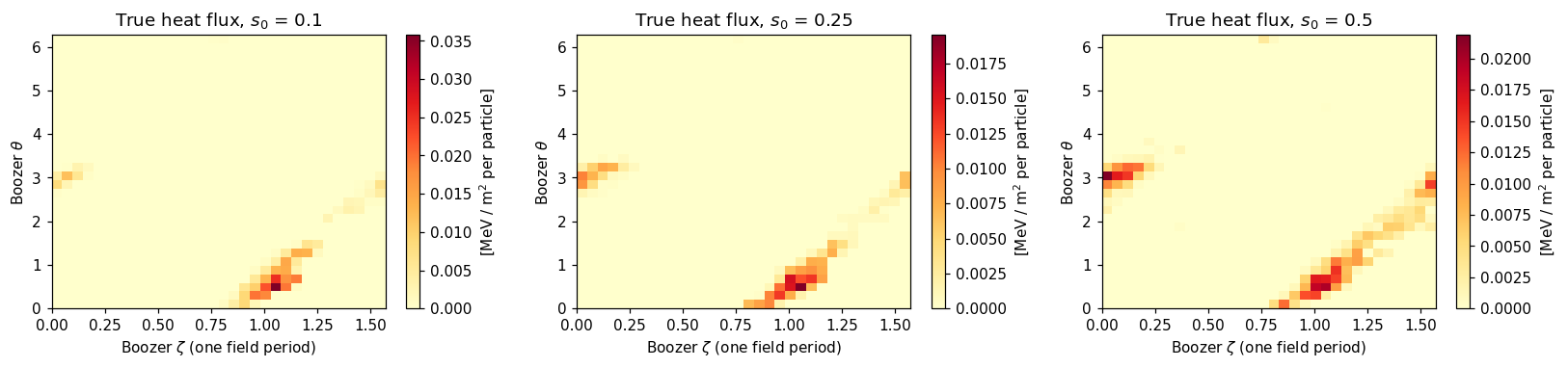
Heat flux on the plasma boundary

Lost particles strike the plasma boundary at their final Boozer angles zeta_end (\(\zeta_B\)) and theta_end (\(\theta_B\)). lost_particles() returns the strike points of the particles born on one surface, and their energies. A particle lost at time \(t_\text{loss}\) carries the energy \(E = 3.5\,\text{MeV} \cdot e^{-2 t_\text{loss} / \tau_s}\), where \(\tau_s\) is the slowing-down time, which we approximate by \(t_\text{max} = 0.1\) s:

zeta, theta, energy, n_launched = bb.lost_particles(rec, s0=0.1)
print(f"{len(zeta)} of the {n_launched} particles born on s = 0.1 are lost")

binned_heat_flux() folds the strike points of all field periods into one, bins their energy, and divides each bin by its area on the boundary, computed from R_boozer, Z_boozer and nu_boozer at \(s = 1\). The result is the heat flux \(Q\) in MeV/m² per launched particle:

Q = bb.binned_heat_flux(zeta, theta, energy, n_launched, rec, resolution=32)
print(Q.shape, f"peak {Q.max():.3g} MeV/m^2 per particle")    # (zeta bin, theta bin)

To get W/m², multiply \(Q\) by an alpha birth rate (particles per second) and by \(1.602 \times 10^{-13}\) J/MeV.

plot_heat_flux() draws the heat flux of the particles born on each surface:

bb.plot_heat_flux(rec)

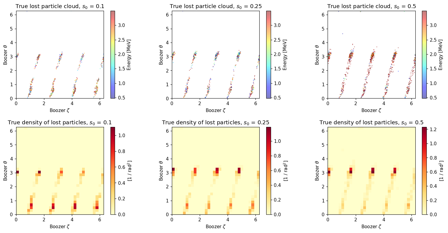
We can also plot where the lost particles strike the boundary, colored by their energy, and the density of the strike points, with plot_strike_points():

bb.plot_strike_points(rec)

Next: Loading trajectory data →