Fitting a surrogate model

Tracing alpha particles is expensive. This tutorial fits a cheap surrogate model that predicts a stellarator’s alpha-particle loss fraction from its shape and profiles, using scikit-learn. It trains on a file from the train split and evaluates on a file from the test split.

pip install scikit-learn

Download at least one train and one test confinement file from the Download Data page into a folder, here BoSS/. The split is part of each file name, so stellarators in a test file are never seen in training.

Features

Each stellarator is described by a feature vector that stacks its plasma boundary, its pressure and current profiles, its number of field periods, and the toroidal flux at its boundary. load() reads chosen fields of every stellarator in a list of files:

import h5py
import numpy as np

import boss_bench as bb

FEATURES = [
    "boundary_xyz",                               # boundary points [m]
    "pressure",                                   # pressure profile [Pa]
    "toroidal_current",                           # toroidal current profile [A]
    "nfp",                                        # number of field periods
    "toroidal_flux_edge",                         # toroidal flux at the boundary [Wb]
]

def build_features(path):
    """Feature matrix, one row per stellarator: the FEATURES side by side."""
    data = bb.load([path], FEATURES)
    cols = [data[name].reshape(len(data[name]), -1) for name in FEATURES]   # scalars become one column
    return np.concatenate(cols, axis=1).astype(np.float64)

Targets

The target is the loss fraction of the 5,000 particles born on the surface \(s_0 = 0.1\), as in the surrogate benchmark (loss_fraction()). The particle arrays are large, so read them in chunks:

def loss_fractions(path, s0=0.1, chunk=256):
    """(n_stellarators,) fraction of the particles born on s0 that are lost."""
    with h5py.File(path, "r") as f:
        t_max = f["t_max"][:]
        y = np.empty(len(t_max))
        for a in range(0, len(y), chunk):
            b = a + chunk
            y[a:b] = bb.loss_fraction(f["confinement_time"][a:b], t_max[a:b], f["s_init"][a:b], s0)
    return y

def load_split(path):
    return build_features(path), loss_fractions(path)

X_train, y_train = load_split(bb.list_files("BoSS", "confinement", "train")[0])
X_test, y_test = load_split(bb.list_files("BoSS", "confinement", "test")[0])
print(X_train.shape, X_test.shape)

To train on more data, load several train files and stack them with np.concatenate.

Fit

The features have very different scales (meters, pascals, amperes, webers), so standardize them first. The 5,043 boundary coordinates are strongly correlated, so a principal component analysis (PCA) compresses them before a gradient-boosted tree model does the regression:

from sklearn.decomposition import PCA
from sklearn.ensemble import HistGradientBoostingRegressor
from sklearn.pipeline import make_pipeline
from sklearn.preprocessing import StandardScaler

model = make_pipeline(
    StandardScaler(),
    PCA(n_components=64, random_state=0),
    HistGradientBoostingRegressor(random_state=0),
)
model.fit(X_train, y_train)

Evaluate

Score the model on the held-out test file, and compare it with the simplest baseline: predicting the mean loss fraction of the training set.

from sklearn.metrics import mean_absolute_error, r2_score

y_pred = np.clip(model.predict(X_test), 0, 1)     # a fraction lies in [0, 1]
baseline = np.full_like(y_test, y_train.mean())

print(f"test MAE: {mean_absolute_error(y_test, y_pred):.3f} "
      f"(baseline {mean_absolute_error(y_test, baseline):.3f})")
print(f"test R^2: {r2_score(y_test, y_pred):.3f}")

A parity plot shows where the model is accurate and where it is not:

import matplotlib.pyplot as plt

fig, ax = plt.subplots(figsize=(4.5, 4.5))
ax.scatter(y_test, y_pred, s=4, alpha=0.4)
ax.plot([0, 1], [0, 1], "k--", lw=1)
ax.set_xlabel("true loss fraction")
ax.set_ylabel("predicted loss fraction")
ax.set_aspect("equal")
fig.tight_layout()

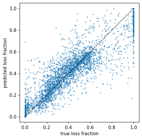
Output for one train file and one test file (about 3,000 stellarators each).

Going further

• Other targets. Predict the loss fraction of the particles born on \(s_0 = 0.25\) or \(0.5\), or the energy they carry out of the plasma with normalized_energy_loss(). See Fast-ion confinement for every particle field.

• Other features. Add any Ideal MHD field, such as iota, modB_boozer or the quasi-symmetry error sqrt_boozer_qs_error, to FEATURES.

• More data. One file holds about 3,000 stellarators; the full train split holds about 154,000.

• The benchmark. The surrogate benchmark scores predictions on every stellarator of the test split; see Benchmarks.