Loading trajectory data

The trajectory files hold full guiding-center orbits of alpha particles. Each file covers up to 40 configurations with 6,000 orbits per configuration, sampled every 1 µs for the first 1 ms. Orbits have different lengths, because a lost particle stops early, so they are stored in a compressed sparse row (CSR) format. traj_data, of shape (n_samples, 5), stacks every sample of every orbit in the file, one row each, with the columns time \(t\) [s], \(s\), Boozer \(\theta\) [rad], Boozer \(\zeta\) [rad] and \(v_\parallel\) [m/s]. Orbit k is rows traj_offsets[k] to traj_offsets[k+1] of traj_data, and the orbits of configuration i are config_offsets[i] to config_offsets[i+1] - 1. The file also holds the configuration fields (uuid, nfp, modB_boozer, iota, …) of its configurations, one row per configuration, exactly as in a confinement file. See Trajectory Data for every field.

Reading one orbit

load_trajectory() reads one orbit, given the configuration, by its row or its uuid, and the index of the orbit:

import h5py
import numpy as np

import boss_bench as bb

# take the first trajectory file of the test split, and one of its configurations
path = bb.list_files("BoSS", "trajectory", "test")[0]
i = 31

with h5py.File(path, "r") as f:
    orbit = bb.load_trajectory(f, i, 1)            # configuration i, its orbit 1
    uuid = f["uuid"].asstr()[i]

t = orbit["t"]
print(f"{uuid}: {len(t)} samples, t from {t[0] * 1e6:.0f} to {t[-1] * 1e6:.1f} us")

The samples are 1 µs apart, starting at \(t = 1\) µs. A lost orbit ends with one extra sample at the time it was lost, which falls between two of those times. The angles are wrapped to \([-\pi, \pi)\).

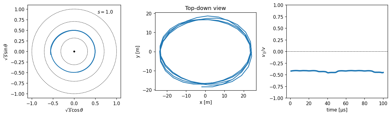
To see where the particle goes, to_xyz() converts the orbit to Cartesian coordinates, using the configuration’s Boozer geometry. Here are its first 100 µs: its path in the poloidal plane, its path seen from above, and its parallel velocity:

import matplotlib.pyplot as plt

with h5py.File(path, "r") as f:
    rec = bb.load_record(f, i)                     # configuration fields, for the geometry
xyz = bb.to_xyz(rec, orbit["s"], orbit["theta"], orbit["zeta"])   # positions [m]

shown = orbit["t"] <= 100e-6                       # the first 100 us
r, theta = np.sqrt(orbit["s"][shown]), orbit["theta"][shown]
fig, axs = plt.subplots(1, 3, figsize=(12, 3.6))
circle = np.linspace(0, 2 * np.pi, 200)
for s_level in (0.1, 0.5, 1.0):                    # flux surfaces, for reference
    axs[0].plot(np.sqrt(s_level) * np.cos(circle), np.sqrt(s_level) * np.sin(circle), "k--", lw=0.6)
axs[0].text(0.55, 0.9, "$s = 1.0$")                # label the outer surface
axs[0].plot(0, 0, "k.")                            # the magnetic axis, s = 0
axs[0].plot(r * np.cos(theta), r * np.sin(theta), lw=1.6)
axs[0].set(xlabel=r"$\sqrt{s}\cos\theta$", ylabel=r"$\sqrt{s}\sin\theta$", aspect="equal")
axs[1].plot(xyz[shown, 0], xyz[shown, 1], lw=1.6)
axs[1].set(xlabel="x [m]", ylabel="y [m]", aspect="equal", title="Top-down view")
axs[2].plot(orbit["t"][shown] * 1e6, orbit["vpar"][shown] / bb.trajectory.V_ALPHA, lw=3)
axs[2].axhline(0, color="k", ls="--", lw=0.6)
axs[2].set(xlabel="time [µs]", ylabel=r"$v_\parallel / v$", ylim=(-1, 1))
fig.tight_layout()

Reading all orbits for one device

read_trajectories() reads all orbits of a configuration at once. traj_data is stored in chunks that run down each column, so this one contiguous read is much faster than reading orbits one at a time. It returns the samples of every orbit on the same time axis, row k being the sample \(k\) µs after the first, in the embedded form that the trajectory benchmark uses,

\[ z = \left(\sqrt{s}\cos\theta,\ \sqrt{s}\sin\theta,\ \cos\varphi,\ \sin\varphi,\ v_\parallel / v_\alpha\right), \]

with \(\theta\) and \(\varphi\) the Boozer poloidal and toroidal angles, and \(v_\alpha\) the speed of a 3.5 MeV alpha particle (embed_state() computes \(z\) from a state):

with h5py.File(path, "r") as f:
    orbits = bb.read_trajectories(f, i)            # by row, or by uuid

z = orbits["z"]
print(z.shape)                                     # (n_orbits, 1000, 5)

A lost orbit stops early: its rows after its last regular sample are NaN, and n_valid counts the rows that are filled. Its final sample, at the time it was lost, falls between rows, so it is not in z; that time is in t_loss instead.

Which orbits are lost

A particle that leaves the plasma within the 1 ms window stops early, at \(s \ge 0.98\), where the integrator stops it. t_loss holds the time it was lost, and NaN for particles that are still confined at 1 ms:

t_loss = orbits["t_loss"]
print(f"lost within 1 ms: {np.isfinite(t_loss).mean():.3f}")
print(f"lost before their first sample: {np.sum(orbits['n_valid'] == 0)}")

Plotting rollouts

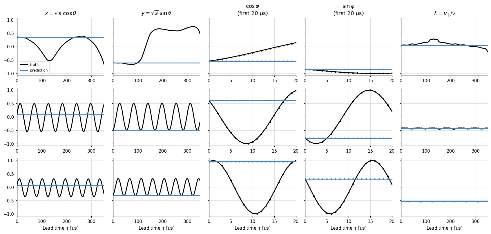
The trajectory benchmark asks a model to predict \(z\) from the first sample of an orbit. plot_rollouts() draws true orbits against predicted ones, one row per orbit and one column per channel of \(z\). Here the “model” predicts that every particle stays at its first sample:

shown = np.flatnonzero(np.isnan(orbits["t_loss"]))[:3]  # three orbits that stay confined
z_pred = np.repeat(z[:, :1], z.shape[1], axis=1)       # every state stays at the first sample
bb.plot_rollouts(z[shown], z_pred[shown])

Joining trajectory and confinement data

rec, read above with load_record(), holds the configuration fields from the trajectory file. To pair the orbits with the confinement results of the same configuration, look for its uuid in the confinement files of the same split:

for conf_path in bb.list_files("BoSS", "confinement", "test"):
    with h5py.File(conf_path, "r") as g:
        if rec["uuid"] in g["uuid"].asstr()[:]:
            conf = bb.load_record(g, rec["uuid"])  # the same configuration, with its 15,000 particles
            break

ct, t_max, s_init = conf["confinement_time"], conf["t_max"], conf["s_init"]
print(f"loss fraction of the particles born on s = 0.1: {bb.loss_fraction(ct, t_max, s_init, 0.1):.3f}")

Next: Fitting a surrogate model →