Using the heat-flux model#
This tutorial predicts the location of lost fast ions on the plasma boundary, with the IID baseline of the paper’s heat-flux task. We show how to compute the heat flux and plot it, for a stellarator from the test split, then how to predict on a new design.
Install the package with its models:
pip install "boss-bench[models]"
Now download and load the model using the convenience functions from boss-bench:
from boss_bench import models
from boss_bench.models import HeatFluxModel

path = models.download("heat_flux", "BoSS-models/heat_flux")
model = HeatFluxModel.load(path)
A stellarator from the test split#
Download confinement_data_test_split_00000.hdf5 from the
Download Data page into a folder, here BoSS/, and load a device.
sample() predicts the loss fraction of
the particles born on one surface \(s_0\), and samples the strike points of the lost
ones: their Boozer angles and energies, one per predicted lost particle of the 5,000
launched:
import h5py

import boss_bench as bb

path = bb.list_files("BoSS", "confinement", "test")[0]
with h5py.File(path, "r") as f:
    record = bb.load_record(f, 0)

zeta, theta, energy, loss_fraction = model.sample(record, s0=0.1, seed=0)
print(f"{len(zeta)} strike points, predicted loss fraction {loss_fraction:.3f}")
1273 strike points, predicted loss fraction 0.255
lost_particles() gives the true strike points, which we
scatter next to the predicted ones, colored by energy:
import matplotlib.pyplot as plt

true = bb.lost_particles(
    record["confinement_time"], record["t_max"], record["s_init"],
    record["zeta_end"], record["theta_end"], s0=0.1)
clouds = {"true": true[:3], "predicted": (zeta, theta, energy)}

fig, axes = plt.subplots(1, 2, figsize=(10, 4), sharey=True)
for ax, (name, (z, t, e)) in zip(axes, clouds.items()):
    points = ax.scatter(z, t, c=e, s=2, cmap="jet", vmin=0, vmax=3.5)
    ax.set_title(f"{name} strike points, $s_0$ = 0.1")
    ax.set_xlabel(r"Boozer $\zeta$")
axes[0].set_ylabel(r"Boozer $\theta$")
fig.colorbar(points, ax=axes, label="energy [MeV]")
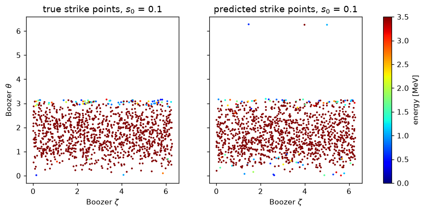
binned_heat_flux() turns strike points into the heat flux
on the boundary, in MeV/m² per launched particle, binned over one field period:
Q = bb.binned_heat_flux(zeta, theta, energy, 5000, record, resolution=32)
print(Q.shape, f"peak {Q.max():.3g} MeV/m^2 per particle")
(32, 32) peak 0.0821 MeV/m^2 per particle
plot_heat_flux() plots the predicted heat flux of each birth
surface next to the true one:
predictions = {}
for s0 in (0.1, 0.25, 0.5):
    predictions[s0] = model.sample(record, s0=s0, seed=0)
bb.plot_heat_flux(record, predictions)
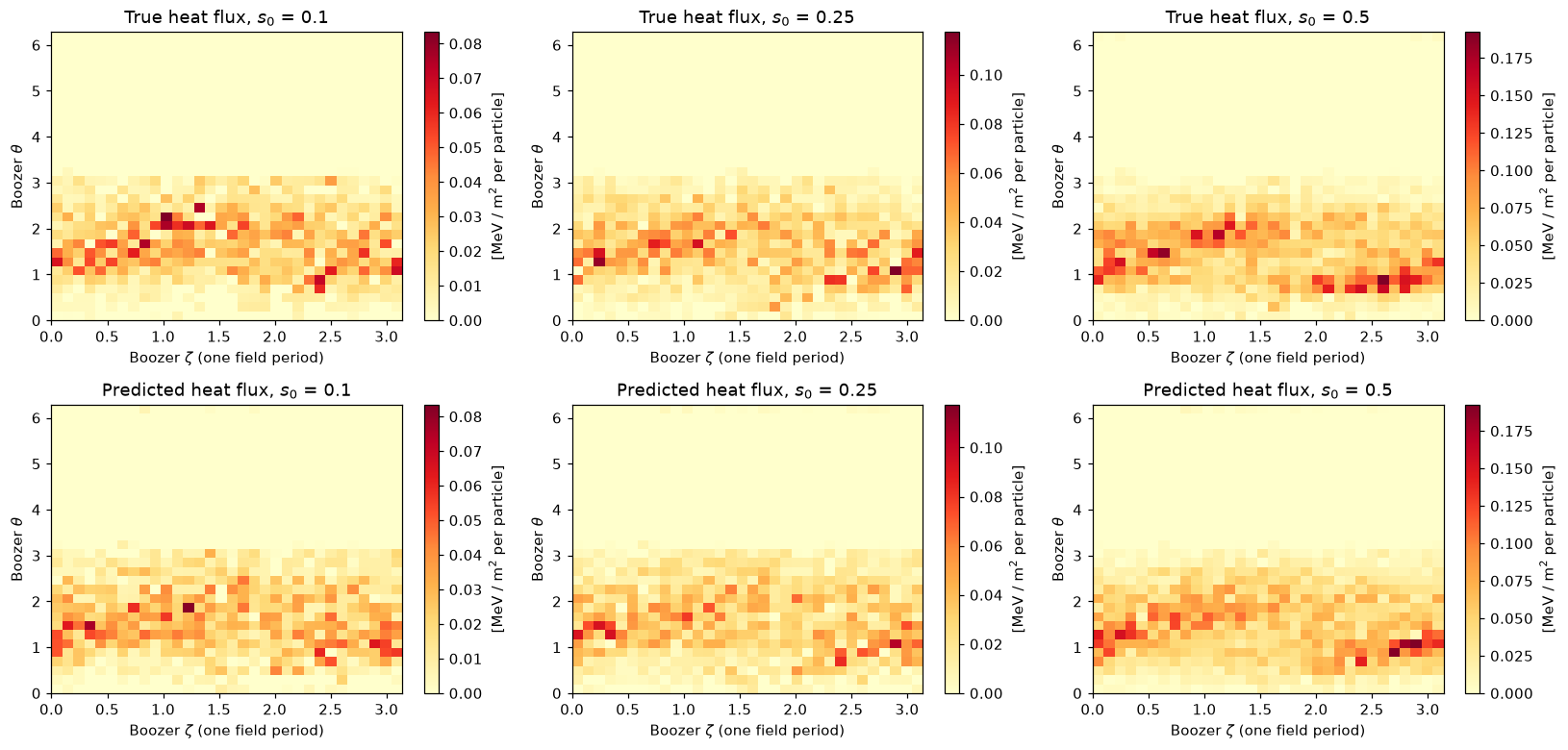
Each prediction (zeta, theta, energy, loss_fraction) is in the format that the
heat-flux benchmark, heat_flux_metrics(), scores.
A new design#
The model can also predict the strike points of a design that is not in the data. As in
Using the loss-fraction surrogate, the boundary is
boundary_xyz = surface.gamma() of a simsopt SurfaceRZFourier with 41 × 41
quadrature points over one field period, and the profiles are evaluated at 15 radial
points linearly spaced from \(s = 10^{-4}\) to 1. The model also needs the rotational
transform; here we use a zero-shear profile, \(\iota = 0.81\) on every surface. The design
is a rotating ellipse at the scale of ARIES-CS, in vacuum (pip install simsopt):
import numpy as np
from simsopt.geo import SurfaceRZFourier

nfp = 3
surface = SurfaceRZFourier(
    nfp=nfp, stellsym=True, mpol=1, ntor=1,
    quadpoints_phi=np.linspace(0, 1 / nfp, 41, endpoint=False),
    quadpoints_theta=np.linspace(0, 1, 41, endpoint=False))
surface.set_rc(0, 0, 7.75)  # major radius [m]
surface.set_rc(1, 0, 1.7)   # minor radius [m]
surface.set_zs(1, 0, 1.7)
surface.set_rc(1, 1, 0.5)   # the rotating ellipse
surface.set_zs(1, 1, -0.5)

design = {
    "boundary_xyz": surface.gamma(),          # (41, 41, 3) [m]
    "nfp": nfp,
    "d_pressure_d_s": np.zeros(15),           # [Pa]
    "iota": np.full(15, 0.81),                # zero shear
    "volume_avg_modB": 5.86,                  # [T]
    "minor_radius": surface.minor_radius(),   # [m]
}
zeta, theta, energy, loss_fraction = model.sample(design, s0=0.1, seed=0)
print(f"{len(zeta)} strike points, predicted loss fraction {loss_fraction:.3f}")
1544 strike points, predicted loss fraction 0.309
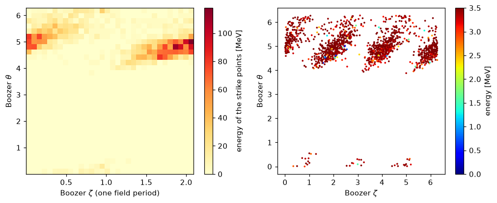
binned_heat_flux() divides by the area of each bin on the
boundary, which it computes from the Boozer coordinates of the boundary (R_boozer,
Z_boozer and nu_boozer, from booz_xform). Without computing the Boozer coordinates,
we plot the energy that the strike points deposit in each bin, with the field periods
folded into one, next to the strike points themselves:
folded = zeta % (2 * np.pi / nfp)  # the field periods folded into one
fig, axes = plt.subplots(1, 2, figsize=(11, 4))
h = axes[0].hist2d(folded, theta, bins=32, weights=energy, cmap="YlOrRd")
fig.colorbar(h[3], ax=axes[0], label="energy of the strike points [MeV]")
axes[0].set_xlabel(r"Boozer $\zeta$ (one field period)")
points = axes[1].scatter(
    zeta, theta, c=energy, s=2, cmap="jet", vmin=0, vmax=3.5)
fig.colorbar(points, ax=axes[1], label="energy [MeV]")
axes[1].set_xlabel(r"Boozer $\zeta$")
for ax in axes:
    ax.set_ylabel(r"Boozer $\theta$")